In [2]:
Image(filename='fig_boxes_map.png')
Out[2]:

# Author: Arthur Prigent
# Email: arthur.prigent@univ-brest.fr

#### DATA ####
# https://downloads.psl.noaa.gov/Datasets/
from functions import *
import warnings
warnings.filterwarnings("ignore")
from IPython.display import Image
2026-07-08 13:50:11.705902
Image(filename='fig_boxes_map.png')
print(str(now)[:16])
2026-07-08 13:50
path_data = 'http://psl.noaa.gov/thredds/dodsC/Datasets/COBE2/sst.mon.mean.nc'
(ssta_atl3_norm_cobe,ssta_aba_norm_cobe,
 ssta_nino34_norm_cobe,ssta_dni_norm_cobe,
 ssta_cni_norm_cobe,ssta_nni_norm_cobe,iod_cobe) = read_data_compute_anomalies(path_data)
#path_oi = 'https://psl.noaa.gov/thredds/dodsC/Datasets/noaa.oisst.v2/'
#path_oi = 'http://psl.noaa.gov/thredds/dodsC/Datasets/noaa.oisst.v2.highres/'
#(ssta_atl3_norm_oi,ssta_aba_norm_oi,
# ssta_nino34_norm_oi,ssta_dni_norm_oi,
# ssta_cni_norm_oi,ssta_nni_norm_oi,iod_index) = read_data_compute_anomalies_oi(path_oi)
path_ersstv5 = 'https://psl.noaa.gov/thredds/dodsC/Datasets/noaa.ersst.v5/sst.mnmean.nc'
(ssta_atl3_norm_ersst,ssta_aba_norm_ersst,
 ssta_nino34_norm_ersst,ssta_dni_norm_ersst,
 ssta_cni_norm_ersst,ssta_nni_norm_ersst,iod_ersst) = read_data_compute_anomalies_ersstv5(path_ersstv5)
plot_anomalies(ssta_atl3_norm_cobe,
               ssta_aba_norm_cobe,
               ssta_nino34_norm_cobe,
               ssta_dni_norm_cobe,
               ssta_cni_norm_cobe,
               ssta_nni_norm_cobe)

#plot_anomalies(ssta_atl3_norm_oi,
#               ssta_aba_norm_oi,
#               ssta_nino34_norm_oi,
#               ssta_dni_norm_oi,
#               ssta_cni_norm_oi,
#               ssta_nni_norm_oi)
plot_anomalies(ssta_atl3_norm_ersst,
               ssta_aba_norm_ersst,
               ssta_nino34_norm_ersst,
               ssta_dni_norm_ersst,
               ssta_cni_norm_ersst,
               ssta_nni_norm_ersst)

ncep_data = 'https://psl.noaa.gov/thredds/dodsC/Datasets/ncep.reanalysis/Monthlies/surface/uwnd.mon.mean.nc'
uwnda_atl4_norm = read_compute_anomalies_uwind_plot(ncep_data)

Methodology inspired from : Fontaine and Louvet (2006)
and with SI the precipitation averaged over 0$^\circ$N-7.5$^\circ$N; 10$^\circ$W-10$^\circ$E
--> NI and SI are then standardized i.e. NI$_{std}$ = NI/(std(NI))
--> a 5-pentad running mean is then apply to the WAMOI time series
path_cmap = 'http://psl.noaa.gov/thredds/dodsC/Datasets/cmap/rt/precip.pentad.mean.rt.nc'
plot_wamoi(path_cmap)
(27, 73)

Sact = $\int_{A(x)} He(25^{\circ}C-SST(x))dA$
where He is the Heaviside function (He = 1 when SST < 25$^{\circ}$C and 0 otherwise). The SST index expresses the intensity of the cooling in the ACT and is defined point by point by subtracting the SST for each grid point from a SST of 25$^{\circ}$C (so that SSTs below 25$^{\circ}$C imply a positive index) inside the domain A, 30$^{\circ}$W–12$^{\circ}$E and 5$^{\circ}$S–5$^{\circ}$N.
path_ersstv5 = 'https://psl.noaa.gov/thredds/dodsC/Datasets/noaa.ersst.v5/'
sst = read_data_ACT_week_plot_ersstv5(path_ersstv5)

The realtime AMM index is defined following the method of Chiang and Vimont (2004). The AMM spatial structure is defined via applying Maximum Covariance Analysis (MCA; Bretherton et al. 1992) is to tropical Atlantic SST and 10m winds over ocean regions between 75E and 15W, 21S to 32N. Data are obtained from the NCEP-NCAR Reanalysis (Kalnay et al. 1996), from NOAA ESRL. The spatial resolution is reduced by averaging three points in the zonal direction, and two points in the latitudinal direction, resulting in approximately 3.8deg latitude by 5.6deg longitude resolution over the region. Next, the seasonal cycle is removed, data are detrended, a three month running mean is applied to the data, and the equatorial Pacific Cold Tongue Index (SST averaged over 180-90W, 6S-6N) is removed (via linear regression) from all points. Finally, the data are weighted by the square root of the cosine of latitude, and the covariance matrix is formed between SST and winds (note the wind fields are appended to each other so the wind state vector has twice as many points as the SST state vector). The covariance matrix is decomposed via Singular Value Decomposition, and the leading statistical mode form the AMM SST and Wind patterns. The time period over which the patterns are computed is frozen as the 1950-2005 time period so that the patterns do not change as the index is being updated.
data_amm = 'https://psl.noaa.gov/data/timeseries/monthly/AMM/ammsst.data'
amm_plot_new(data_amm)

#data_amo= 'https://www1.ncdc.noaa.gov/pub/data/cmb/ersst/v5/index/ersst.v5.amo.dat'
#plot_amo_new(data_amo)
ncep_data_slp = 'https://psl.noaa.gov/thredds/dodsC/Datasets/ncep.reanalysis.derived/surface/slp.mon.mean.nc'
plot_slp(ncep_data_slp)

plot_IOD(iod_cobe)

plot_IOD(iod_ersst)

_,_,table_atl3_w,table_atl3_c = create_table_event_new(ssta_atl3_norm_ersst)
table_atl3_w
| Start date | End date | Duration | Mean SSTa | Cumul SSTa | Max SSTa | Date max SSTa | |
|---|---|---|---|---|---|---|---|
| 0 | 1984-06 | 1984-10 | 4 | 1.65 | 6.59 | 2.18 | 1984-09 |
| 1 | 1987-06 | 1987-10 | 4 | 2.01 | 8.06 | 2.89 | 1987-07 |
| 2 | 1988-03 | 1988-09 | 6 | 2.20 | 13.20 | 3.18 | 1988-07 |
| 3 | 1989-06 | 1989-10 | 4 | 1.23 | 4.93 | 1.37 | 1989-08 |
| 4 | 1993-09 | 1994-01 | 4 | 1.43 | 5.72 | 2.11 | 1993-11 |
| 5 | 1995-05 | 1995-08 | 3 | 1.48 | 4.43 | 1.60 | 1995-06 |
| 6 | 1996-05 | 1996-08 | 3 | 1.80 | 5.41 | 2.56 | 1996-06 |
| 7 | 1997-12 | 1998-03 | 3 | 1.49 | 4.46 | 1.57 | 1998-01 |
| 8 | 1998-06 | 1998-09 | 3 | 1.34 | 4.03 | 1.63 | 1998-06 |
| 9 | 2016-10 | 2017-01 | 3 | 1.23 | 3.69 | 1.45 | 2016-11 |
| 10 | 2019-11 | 2020-03 | 4 | 2.14 | 8.56 | 2.39 | 2020-01 |
| 11 | 2021-06 | 2021-10 | 4 | 2.09 | 8.36 | 2.54 | 2021-07 |
| 12 | 2024-02 | 2024-05 | 3 | 2.12 | 6.37 | 2.72 | 2024-03 |
table_atl3_c
| Start date | End date | Duration | Mean SSTa | Cumul SSTa | Max SSTa | Date max SSTa | |
|---|---|---|---|---|---|---|---|
| 0 | 1982-06 | 1982-10 | 4 | -1.38 | -5.52 | -1.76 | 1982-07 |
| 1 | 1991-11 | 1992-02 | 3 | -1.60 | -4.81 | -1.85 | 1991-11 |
| 2 | 1992-04 | 1992-10 | 6 | -1.72 | -10.30 | -2.46 | 1992-05 |
| 3 | 1996-11 | 1997-07 | 8 | -1.73 | -13.82 | -2.59 | 1997-06 |
| 4 | 2000-06 | 2000-12 | 6 | -1.22 | -7.34 | -1.28 | 2000-11 |
| 5 | 2001-11 | 2002-02 | 3 | -1.87 | -5.60 | -2.39 | 2001-12 |
| 6 | 2004-04 | 2004-07 | 3 | -1.37 | -4.12 | -1.59 | 2004-04 |
| 7 | 2005-05 | 2005-08 | 3 | -2.55 | -7.66 | -3.20 | 2005-06 |
| 8 | 2009-07 | 2009-12 | 5 | -1.31 | -6.57 | -1.65 | 2009-08 |
| 9 | 2011-12 | 2012-08 | 8 | -1.67 | -13.32 | -2.05 | 2012-02 |
| 10 | 2013-07 | 2014-01 | 6 | -1.27 | -7.60 | -1.51 | 2013-09 |
| 11 | 2015-06 | 2015-09 | 3 | -1.17 | -3.51 | -1.37 | 2015-08 |
| 12 | 2025-06 | 2025-09 | 3 | -1.77 | -5.32 | -1.90 | 2025-07 |
_,_,table_aba_w,table_aba_c = create_table_event_new(ssta_aba_norm_ersst)
table_aba_w
| Start date | End date | Duration | Mean SSTa | Cumul SSTa | Max SSTa | Date max SSTa | |
|---|---|---|---|---|---|---|---|
| 0 | 1984-02 | 1984-10 | 8 | 2.34 | 18.72 | 3.07 | 1984-03 |
| 1 | 1991-05 | 1991-08 | 3 | 1.80 | 5.39 | 2.49 | 1991-05 |
| 2 | 1994-10 | 1995-01 | 3 | 1.41 | 4.22 | 1.55 | 1994-10 |
| 3 | 1995-02 | 1995-06 | 4 | 2.61 | 10.43 | 3.42 | 1995-04 |
| 4 | 1996-03 | 1996-07 | 4 | 1.62 | 6.49 | 2.34 | 1996-04 |
| 5 | 1997-10 | 1998-02 | 4 | 1.58 | 6.31 | 1.78 | 1997-12 |
| 6 | 2011-01 | 2011-05 | 4 | 1.78 | 7.13 | 1.94 | 2011-03 |
| 7 | 2019-11 | 2020-02 | 3 | 1.78 | 5.33 | 2.22 | 2019-11 |
| 8 | 2021-05 | 2021-09 | 4 | 1.80 | 7.19 | 2.21 | 2021-06 |
| 9 | 2023-11 | 2024-03 | 4 | 1.40 | 5.60 | 1.93 | 2023-12 |
table_aba_c
| Start date | End date | Duration | Mean SSTa | Cumul SSTa | Max SSTa | Date max SSTa | |
|---|---|---|---|---|---|---|---|
| 0 | 1983-03 | 1983-08 | 5 | -1.40 | -6.99 | -1.83 | 1983-04 |
| 1 | 1991-11 | 1992-02 | 3 | -1.07 | -3.21 | -1.13 | 1991-11 |
| 2 | 1992-03 | 1992-09 | 6 | -1.51 | -9.03 | -1.81 | 1992-03 |
| 3 | 1996-11 | 1997-07 | 8 | -1.99 | -15.91 | -3.07 | 1997-03 |
| 4 | 2001-12 | 2002-03 | 3 | -1.43 | -4.29 | -1.90 | 2002-01 |
| 5 | 2004-03 | 2004-06 | 3 | -2.27 | -6.82 | -3.13 | 2004-04 |
| 6 | 2005-04 | 2005-10 | 6 | -1.57 | -9.40 | -2.67 | 2005-05 |
| 7 | 2010-02 | 2010-05 | 3 | -1.49 | -4.48 | -1.85 | 2010-04 |
| 8 | 2011-06 | 2011-09 | 3 | -1.13 | -3.38 | -1.19 | 2011-08 |
| 9 | 2011-11 | 2012-04 | 5 | -1.77 | -8.83 | -2.43 | 2012-01 |
Figure inspired by the Richter et al., (2013), in which they identify some warm events that can not be explained by previously identify equatorial wind stress forcing.
--> A warm SST event is categorized as a canonical (non-canonical) event when it is preceded by a positive (negative) surface wind anomaly. Hence, canonical events lie in the upper right (in red) and lower left (in blue), and non-canonical events lie in the upper left and lower right (in black) quadrants.
plot_canonical_atlantic_ninos(uwnda_atl4_norm,ssta_atl3_norm_ersst)

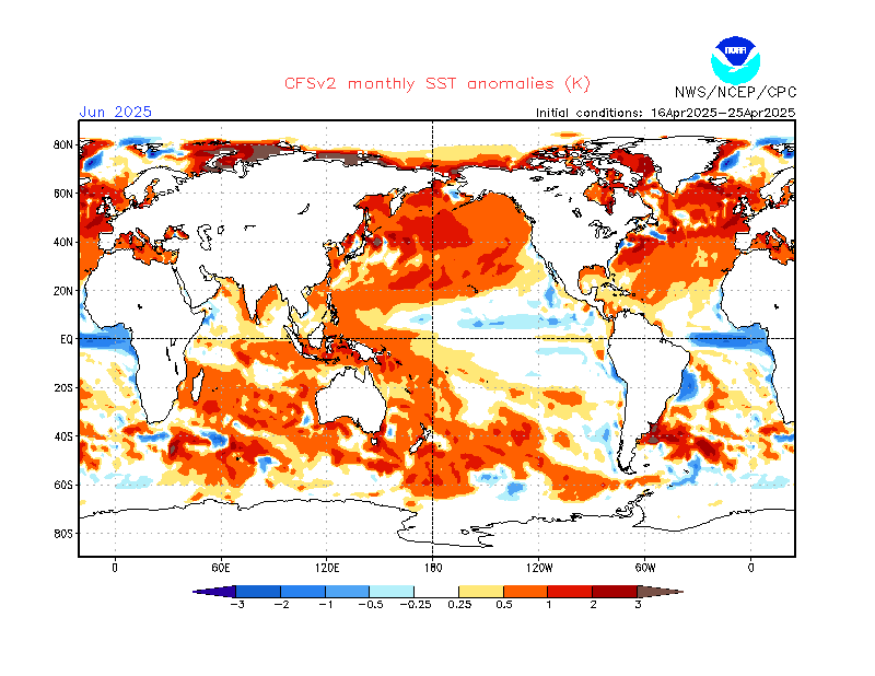
Image(url='https://www.cpc.ncep.noaa.gov/products/CFSv2/imagesInd3/glbSSTMonInd2.gif')
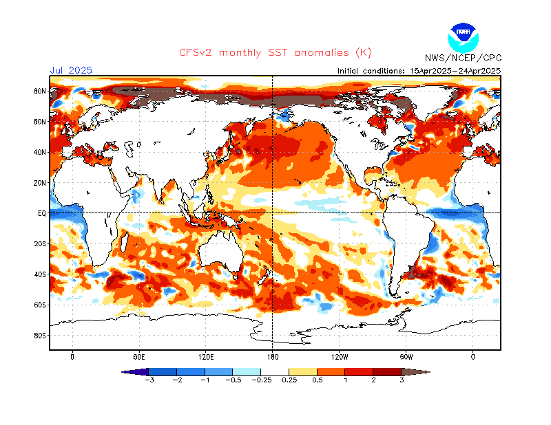
Image(url='https://www.cpc.ncep.noaa.gov/products/CFSv2/imagesInd3/glbSSTMonInd3.gif')
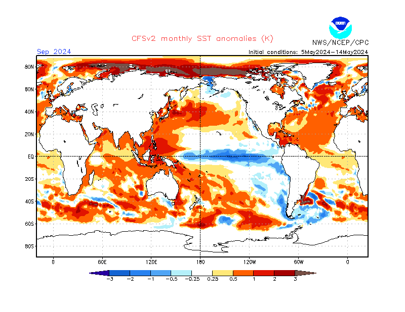
Image(url='https://www.cpc.ncep.noaa.gov/products/CFSv2/imagesInd3/glbSSTMonInd4.gif')
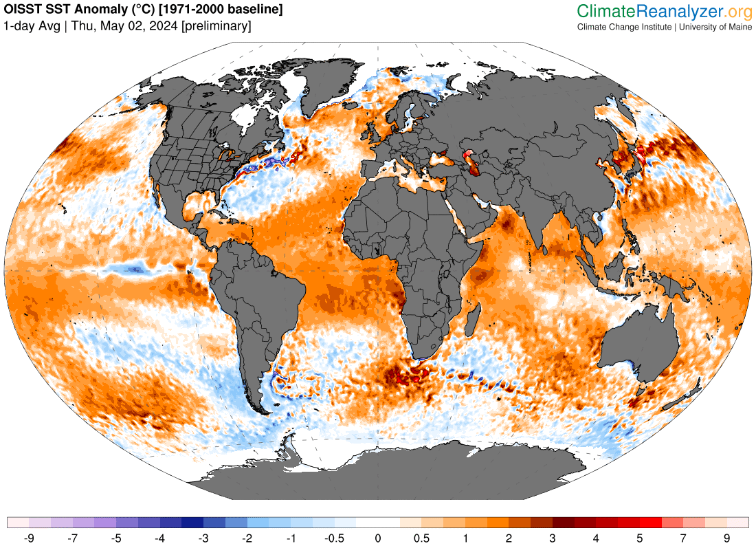
Image(url='https://climatereanalyzer.org/wx/todays-weather/maps/gfs_world-wt_sstanom_d1.png')
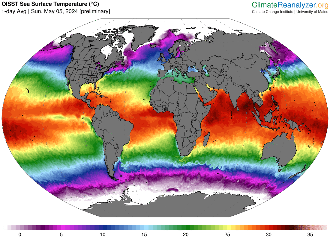
Image(url='https://climatereanalyzer.org/wx/todays-weather/maps/gfs_world-wt_sst_d1.png')
Image(url='https://www.cpc.ncep.noaa.gov/products/GODAS/pent_gif/xz/movie.temp.0n.gif',width=800)
Image(url='https://www.cpc.ncep.noaa.gov/products/GODAS/pent_gif/xy/movie.d20.gif',width=800)